Multiplexed analysis

This tutorial outlines the basics of how multiplexed images can be analyzed in QuPath using the sample LuCa-7color_[13860,52919]_1x1component_data.

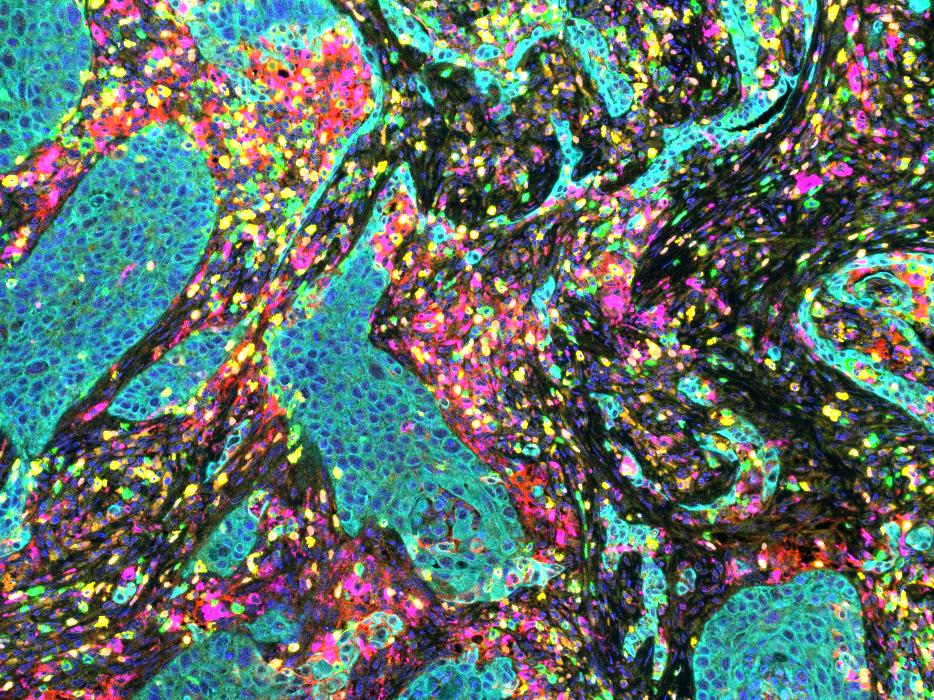
We will focus on the main task of identifying each cell, and classifying the cells according to whether they are positive or not for different markers. Once this has been done, ‘standard’ QuPath commands and scripts can be used to interrogate the data.

Note

If you are looking to quantify stained areas rather than cells or needing to create an annotation before running cell detection then Measuring areas or Pixel classification tutorials may be of interest. Although the examples used in these tutorials are brightfield stains, the methods are the same for fluorescence. When required to enter the “channel” just use the one of interest in your image instead.

This tutorial has three main steps:

1. Detect & measure cells

2. Create classifiers for each marker

3. Combine the classifiers and apply them to cells

But first we have a few routine things we need to take care of so that things can run smoothly.

Step-by-step

Before we begin…

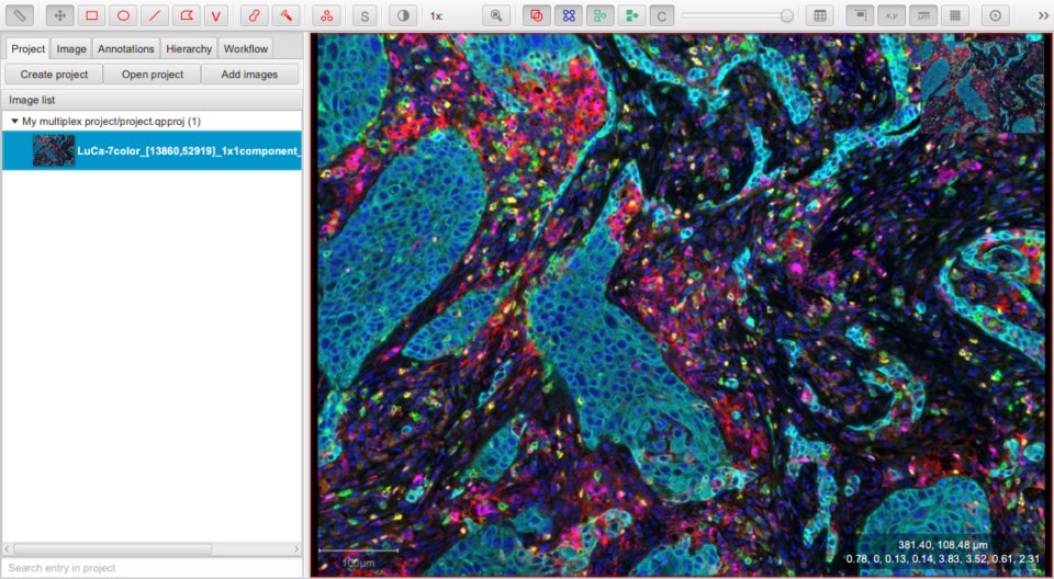
Create a project containing your images

Many things in QuPath work best if you create a Project. Here, it is really necessary so that classifiers generated along the way are saved in the right place to become available later.

Set the image type

As usual when working with an image in QuPath, it is important to ensure the Image type is appropriate. In this case, the best choice is Fluorescence.

Tip

The type Fluorescence can be used even when not exactly true (e.g. for other exotic image types). The main thing is to choose the closest match.

The Fluorescence type here tells QuPath that ‘high pixel values mean more of something’. Choosing Brightfield conveys the opposite message, which would cause problems because cell detection would then switch to looking for dark nuclei on a light background.

Accurate cell detection

Good cell segmentation is really essential for accurate multiplexed analysis. New and improved methods of segmenting cells in QuPath are being actively explored…

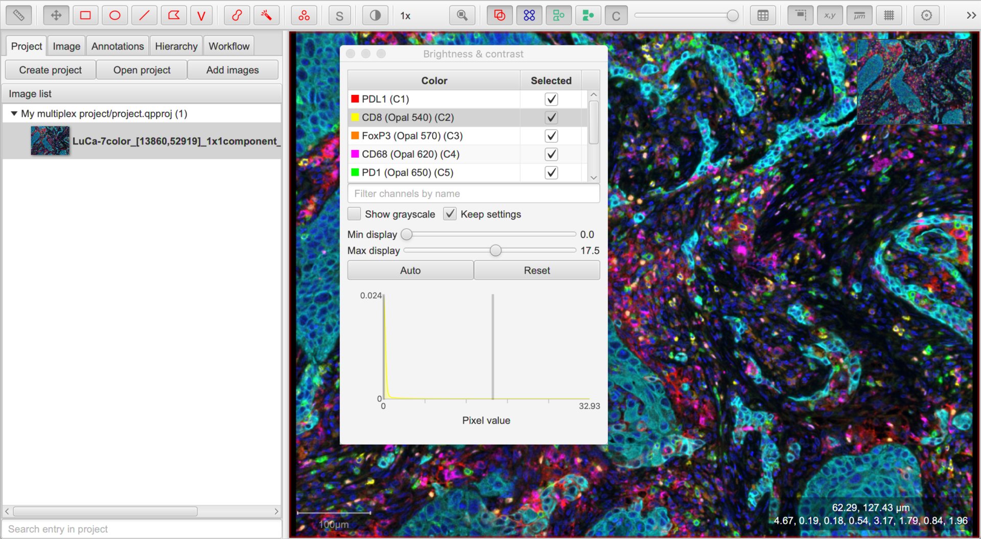
Set up the channel names

The channel names are particularly important for multiplexed analysis, since these typically correspond to the markers of interest. They will also be reused within the names for the cell classifications.

Therefore we usually want them to be short accurate and stripped of any extra text we do not really need.

The names can be seen in the Brightness/Contrast dialog, and edited by double-clicking on any entry to change the channel properties. Here, I would remove any ‘(Opal)’ parts.

Tip

Setting all the channel names individually can be very laborious. Two tricks can help.

1. Outside QuPath (or in the Script editor) create a list of the channel names you want, with a separate line for each name. Copy this list to the clipboard, and then select the corresponding channels in the Brightness/Contrast dialog and press Ctrl + V to paste them.

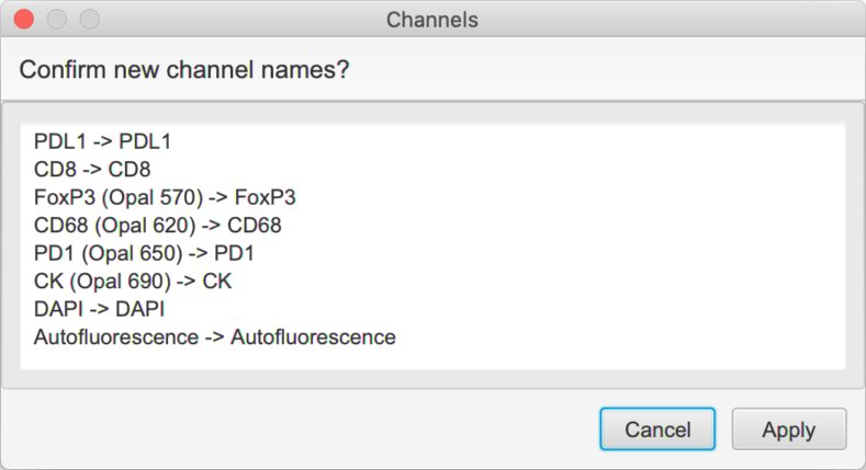
2. Run a script like the following:

setChannelNames(
     'PDL1',
     'CD8',
     'FoxP3',
     'CD68',
     'PD1',
     'CK'
)

Tip

The original names are not lost. You can retrieve them later by going to the Image tab, and double-clicking the row that states Metadata changed: Yes. This allows you to reset all the image metadata to whatever was read originally from the file, including the channel names.

Setting up the classifications

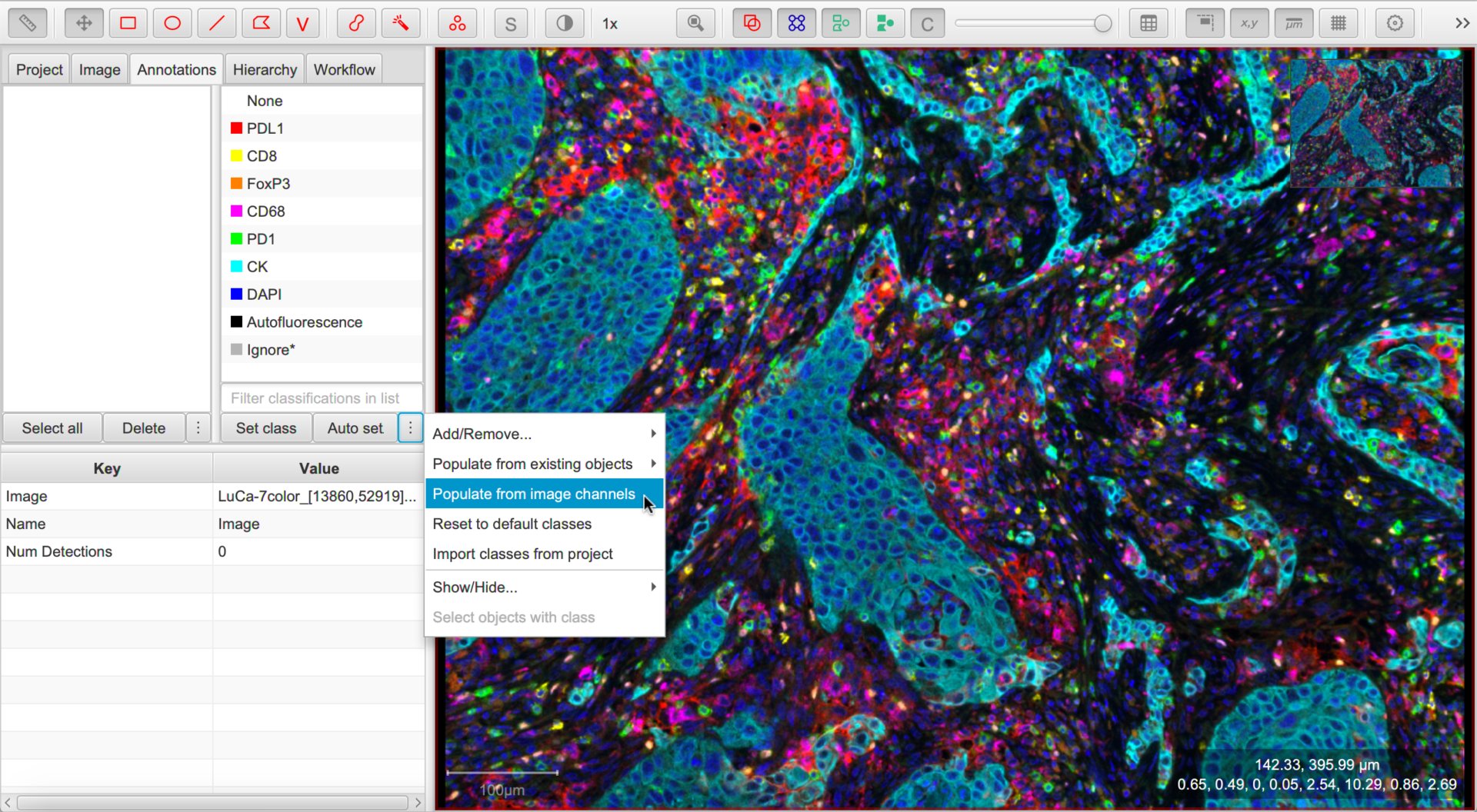
We now want to make the channel names available as classifications.

The classifications currently available are shown under the Annotations tab. You can either right-click this list or select the ⋮ button and choose Populate from image channels to quickly set these.

Detect & measure cells

QuPath’s default Cell detection command can be applied for fluorescence and multiplexed images, not only brightfield.

The key requirement is that a single channel can be used to detect all nuclei. If so, select that channel and explore different parameters and thresholds until the detection looks acceptable.

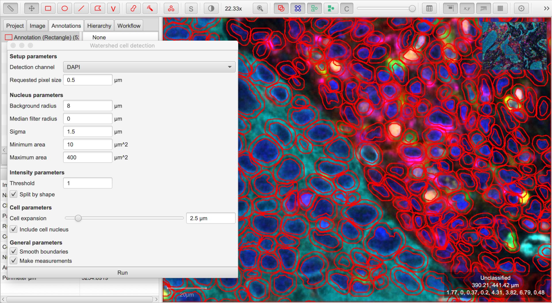
Along with the cell detection, QuPath automatically measures all channels in different cell compartments. Because these measurements are based on the channel names, it is important to have these names established first.

Create a classifier for each marker

The next step involves finding a way to identify whether cells are positive or negative for each marker independently based upon the detections and measurements made during the previous step.

Since QuPath v0.2.0 there are two different ways to do this:

1. Threshold a single measurement (e.g. mean nucleus intensity)

2. Train a machine learning classifier to decide based upon multiple measurements

Both methods are described below. You do not have to choose the same method for every marker, but can switch between the two methods.

Option #1. Simple thresholding

QuPath v0.2.0 introduced a new command, Classify ‣ Object classification ‣ Create single measurement classifier. This gives us a quick way to classify based on the value of one measurement.

As usual, you can consider the options in the dialog box in order from top to bottom, and hover the cursor over each for a short description of what it means.

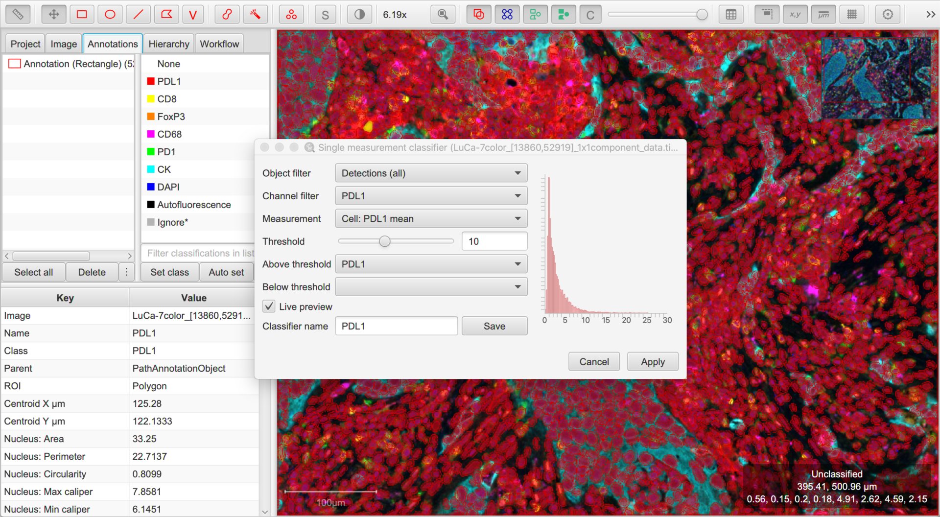
In this case, we can ignore the Object filter (all our detections are cells, so no need to distinguish between them).

The Channel filter will be helpful, because it will help us quickly set sensible defaults for the options below. We should set this to be the first channel we want to use for classification.

Next, we then choose which measurement is relevant for the selected channel using the Measurement drop-down list, and adjust the threshold for that measurement with the Threshold slider.

Cells having measurements with values greater than or equal to the threshold will be assigned the classification selected through the Above threshold drop-down list, and the rest assigned the classification through Below threshold.

Here, we want Above threshold to be the classification for a ‘positive’ cell (i.e. the channel name), and Below threshold should not have a classification at all. We can achieve this by leaving Below threshold to be blank, or alternatively setting it to Unclassified.

To see the effects of any adjustments we make, we can use the Live preview option.

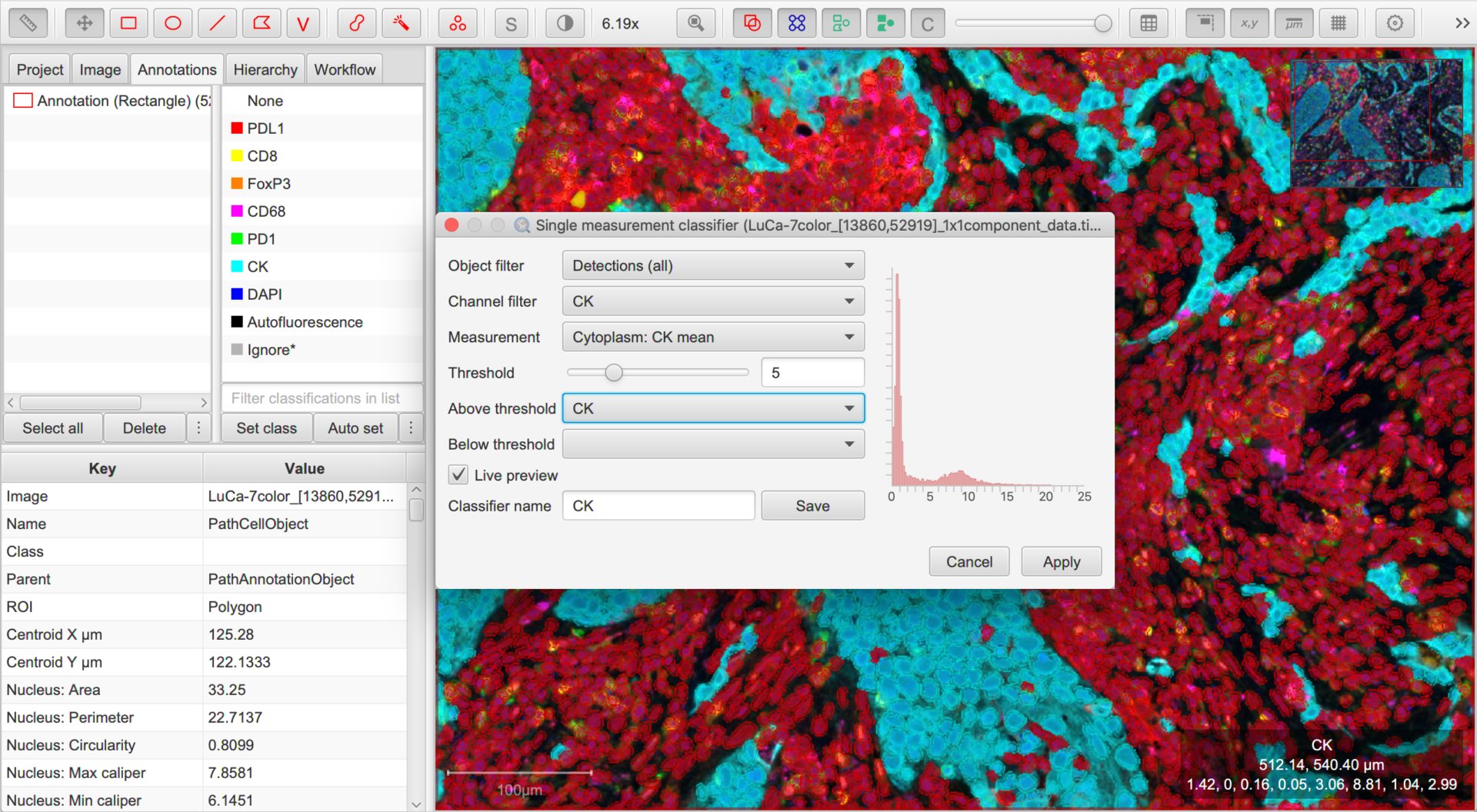
Once you are reasonably content with the results, check (and amend if necessary) the Classifier name and click Save. This will save a classifier with the current settings to the project.

Now you can return to the Channel filter and work through the steps for the other channels.

Option #2. Machine learning

If you are entirely happy with the process above, you can skip this section. But sometimes thresholding a single measurement isn’t sufficient to generate a usable classification - and taking a machine learning approach can help. This process is a bit more involved, but the effort is often worth it.

Create training images

It is very difficult and confusing to try to train multiple classifiers by annotating the same image.

The process is made easier by creating duplicate images within the project for each channel that needs a classifier. To do this, choose Classify ‣ Training Images ‣ Create duplicate channel training images.

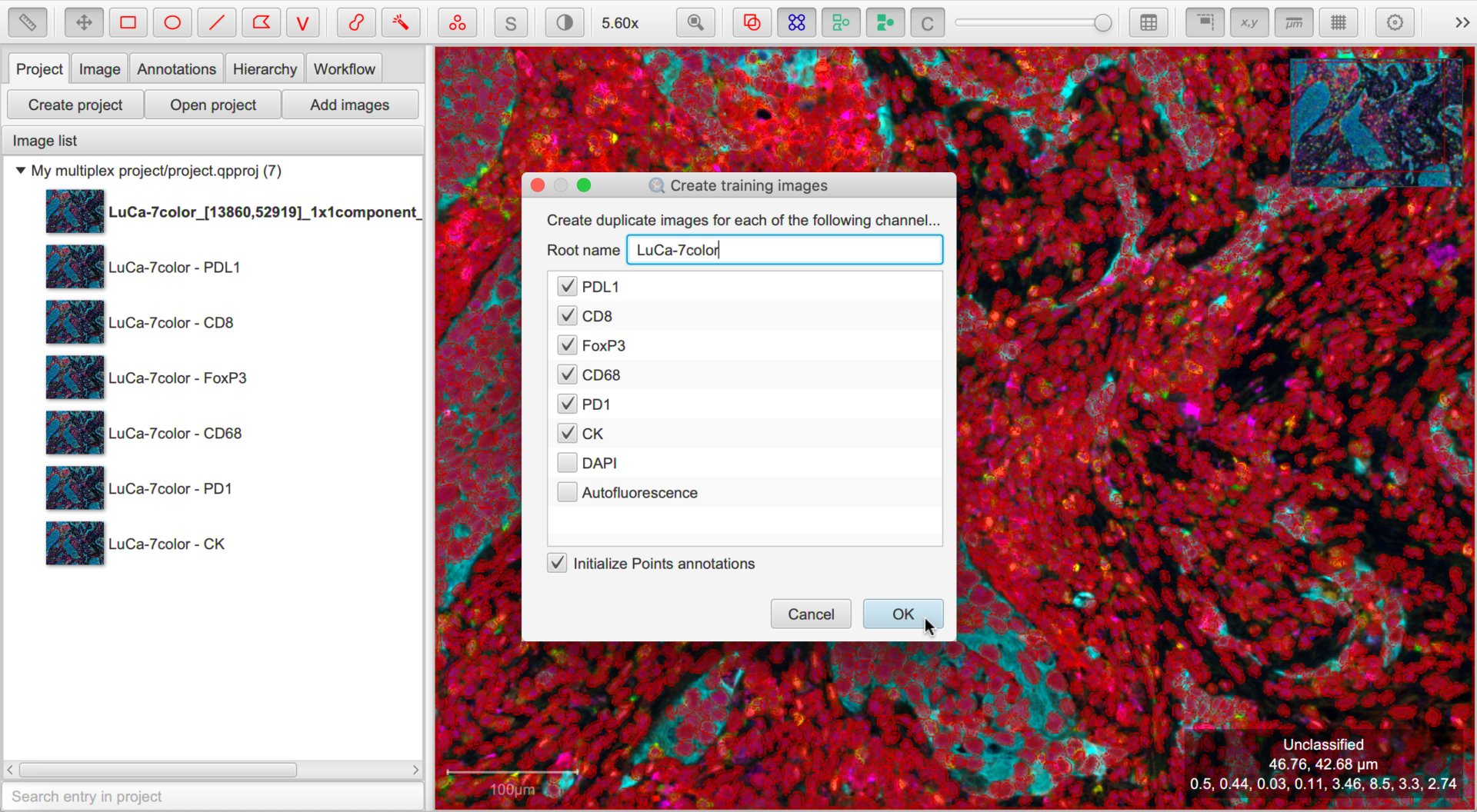
Note

It’s useful to run cell detection before duplicating the images so the detections match!

Tip

It is a good idea to turn the Initialize Points annotation option on… it might help us later.

Train & save classifiers

Now you should have multiple duplicate images in your project, with names derived from the original channel names. Because you ran this after cell detection (right?!), these duplicate images will bring across all the original cells.

We can then proceed with Classify ‣ Object classification ‣ Train object classifier.

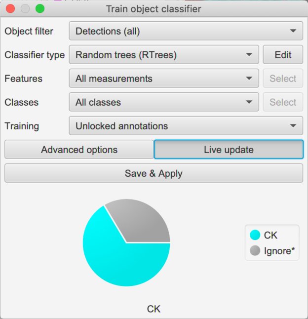
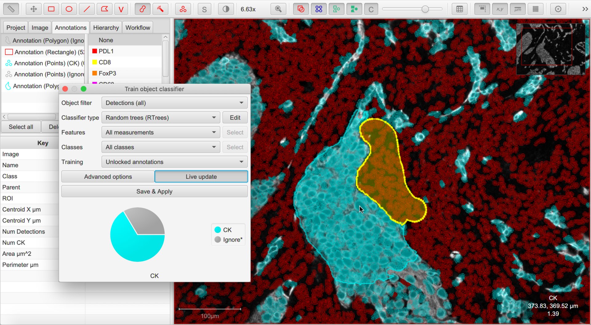
The concepts are similar to those in Cell classification: we annotate the image with points or areas where we know what the classification should be, and assign that classification to our annotations. QuPath then uses the cells identified by these annotations to train a machine learning classifier.

To begin, we should check the options in the dialog box again. We can skip the Object filter, and explore the difference of changing Classifier type later.

Next, we come to Features. In principle, we could train our classifier to use any or all cell measurements as features. This is what the default All measurements option will do.

But here, we probably want to be more selective and restrict the features going into the classifier to only those relevant to the marker of interest

We can do that by choosing Selected measurements and pressing the Select button to specify exactly what we want to use - this gives us full control, but we do need to remember to choose the features separately for every classifier we build (lest we accidentally train classifiers for some markers based on measurements made of completely different markers).

The Filtered by output classes option gives us a fast compromise: measurements will automatically be chosen based upon the names of the classifications we are training. In other words, if we are training a classifier with an output of CD8 then only measurements that contain CD8 somewhere in their name will be counted (or cd8 or cD8 - it’s case-insensitive).

Tip

Be careful if you have markers where one name also appears as part of another name, so that the above simple filter won’t be enough… like CD8, CD88 and CD888.

The Classes option allows us to specify what we are training for. We can leave this to All classes and simply only annotate cells with the classes we care about.

We can also leave Training to be Unlocked annotations, meaning that anything new we draw can be used for training.

With that out of the way, it is time to annotate. We have two main options: points (using the Counting tool) or areas (e.g. using the brush, wand or polygon tools).

The essential thing we must do is assign annotations for ‘positive’ cells with the classification we are interested in (e.g. FoxP3), and ‘negative’ cells with the special classification Ignore*. We shouldn’t use any other classes in the training annotations.

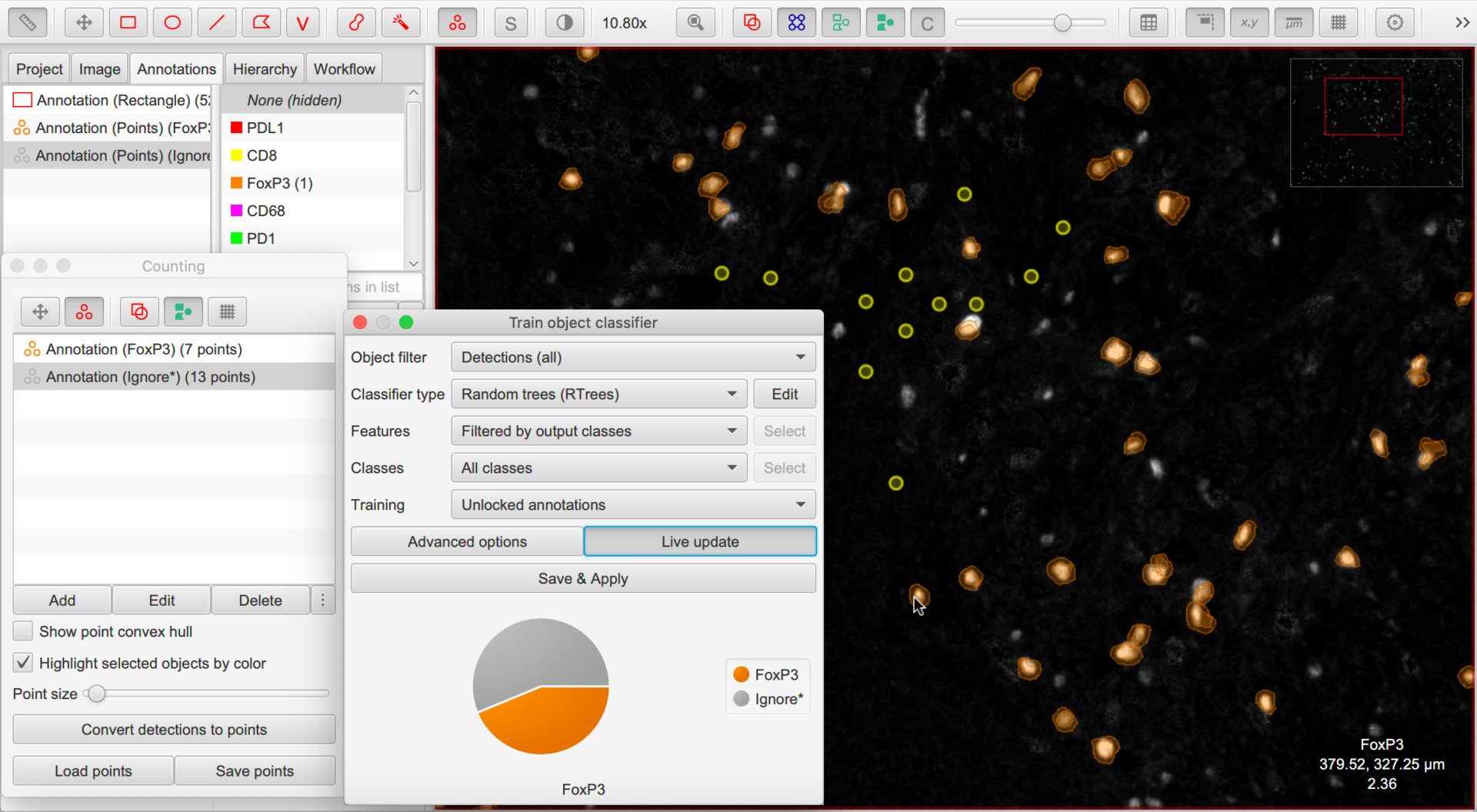
Once you are done with one marker, choose Save & Apply and enter a name to identify your classifier. Then save the image data and open the image associated with the next marker of interest, repeating the process as many times as necessary.

Tip

I find three things helpful when training a single-channel classifier:

• Turn off cells (e.g. press the D shortcut key) most of the time

• Make a single channel visible in grayscale mode using the Brightness/Contrast dialog

• Hide the Unclassified cells when the cells are being displayed for verification - this can be done by right-clicking the unclassified option on the classification list.

You can then proceed to annotate cells, largely free of the distraction of what QuPath had actually previously detected.

Combine the classifiers

At this point, the hard work has been done.

You can return to your original image that you want to classify and choose Classify ‣ Object classification ‣ Load object classifier.

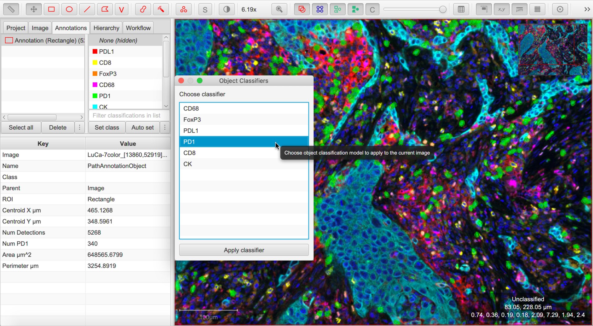
This should display all the classifiers available within the project. Choose any and press Apply classifier to see it in action.

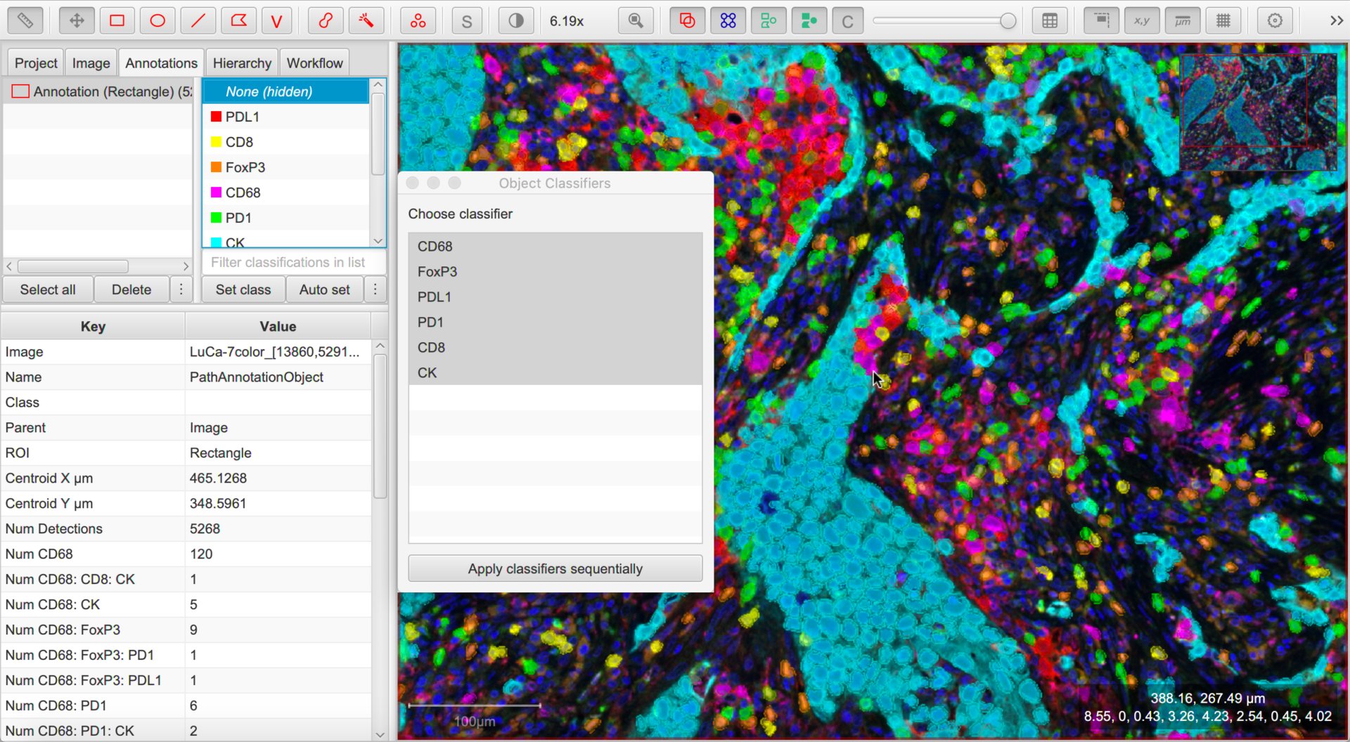
Then, choose any combination of classifiers and press Apply classifiers sequentially to see the effect of all of them upon the image.

Tip

To avoid needing to repeatedly select more than one classifier under Load object classifier, you can create a single ‘combined’ classifier using Classify ‣ Object classification ‣ Create composite classifier.

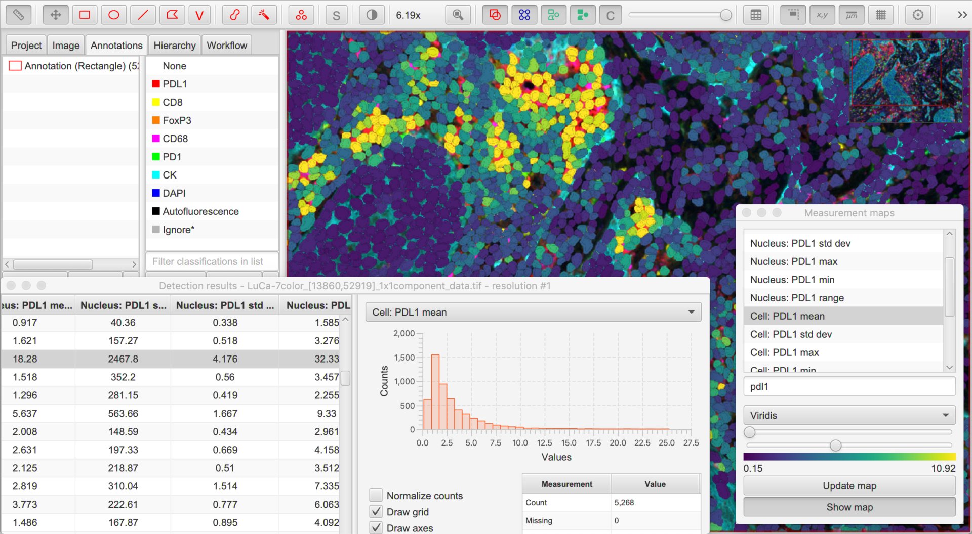
Making sense of it all

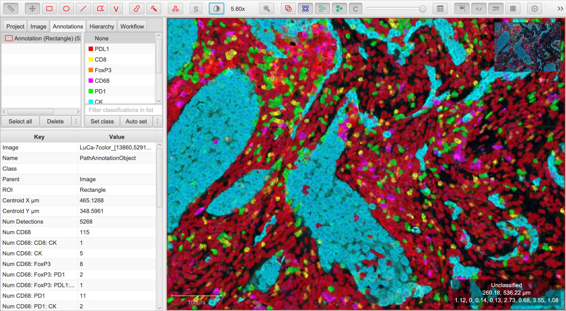
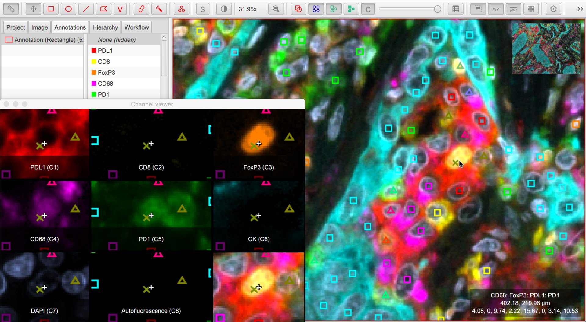
Amidst a blaze of color, it can rapidly become difficult to interpret images. A few things can help:

• The box in the bottom right corner of the viewer now shows not only the mouse location, but also the classification of the object under the cursor.

• View ‣ Show channel viewer makes it possible to see all channels side-by-side. Right-click on the channel viewer to customize its display.

• Right-clicking on the Classifications list under the Annotations tab, you can now use Populate from existing objects ‣ All classes to create a list of all classifications present within the image. The filter box below this list enables quickly finding classifications including specific text. You can then select these, and toggle their visibility by right-clicking or pressing the spacebar.

• Right-click on the image and choose Cells ‣ Centroids only to have another view of the classified cells. Now, the shape drawn for each cell relates to the ‘number of components’ of its classification, while its color continues to depict the specific class. This makes similar-but-not-the-same classifications to be spotted more easily than using (often subtle) color differences alone.

One class or many?

When querying the data, it can be helpful to know that objects in QuPath can ultimately only have a single classification, but this classification can have different pieces.

Therefore when applying multiple classifiers in this way, the single classification in the end is determined by piecing together the individual parts - represented here as Class 1: Class 2: Class 3, for example.

This means that if you compare whether two objects have identical classifications, i.e. cell1.getPathClass() == cell2.getPathClass() this automatically means that all components of the classification are considered.

A script like the following can be used to extract the component parts:

def pathObject = getSelectedObject()
def pathClass = pathObject.getPathClass()
def parts = PathClassTools.splitNames(pathObject.getPathClass())

println(parts)