Density maps
Density maps were originally created to help find ‘hotspots’ for specific applications in pathology (e.g. tumor budding, Ki67 scoring). However, their implementation in QuPath is designed to be much more flexible than that.
In some cases, density maps can even be a replacement for Pixel classification or Superpixels.
Warning
Like most commands in QuPath, Density Maps are currently calculated only in 2D. And, like many other commands, you should create Density Maps within a project if you want to reuse them later.
Getting started with density maps
The starting point for creating a density map is usually to generate and classify a large number of detections on an image. Here, we use do this by following the steps in Cell detection and Cell classification.
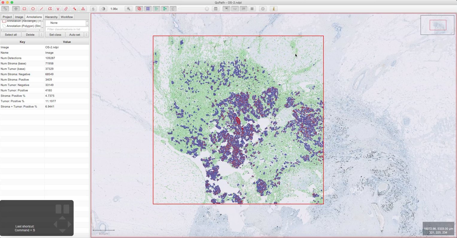
Ki67 image with classified cells
Then launch the density map command with .
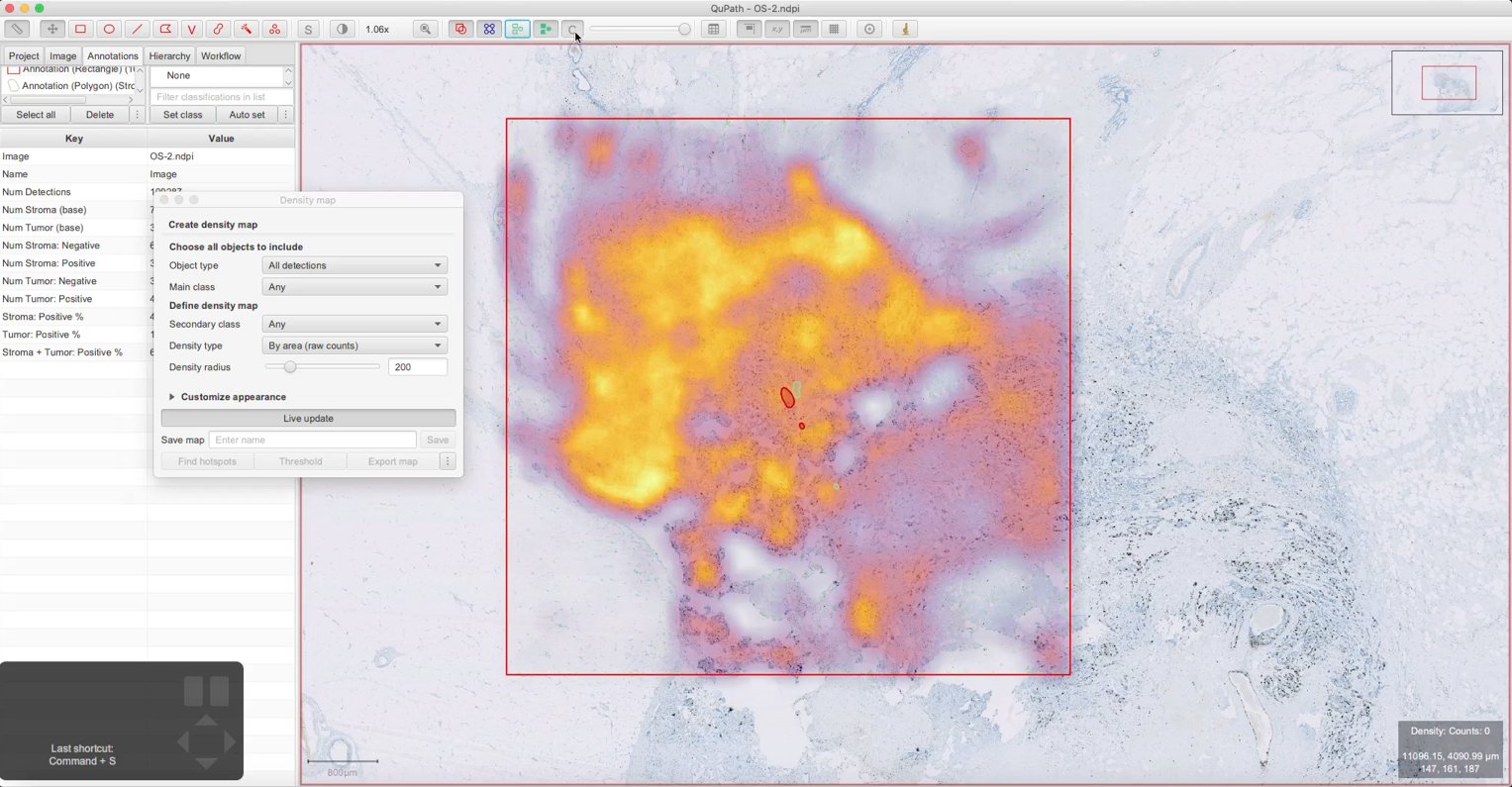
Original density map
The density map is effectively a lower-resolution image in which each pixel relates to the density of objects within a defined radius. This can be used to find areas containing a high density of those objects, either as contours with irregular shapes or circular hotspots of a fixed size.
The display of the map is toggled in the same way as a threshold/pixel classification: using the C shortcut key or C button in QuPath’s toolbar.
Tip
You will probably need to toggle off the detections to see the density map more clearly.
You can do this by pressing the D shortcut or  toolbar button.
Customizing density maps
The density map options dialog aims to guide you through the parameters you might want to adjust. Hovering your mouse over any option should provide some help text.
Choosing objects to include
The Object type and Main class define which objects will contribute to the density map in some way.
Left to the defaults, the density map will make use of all detection objects (which includes cells) regardless of their classification.
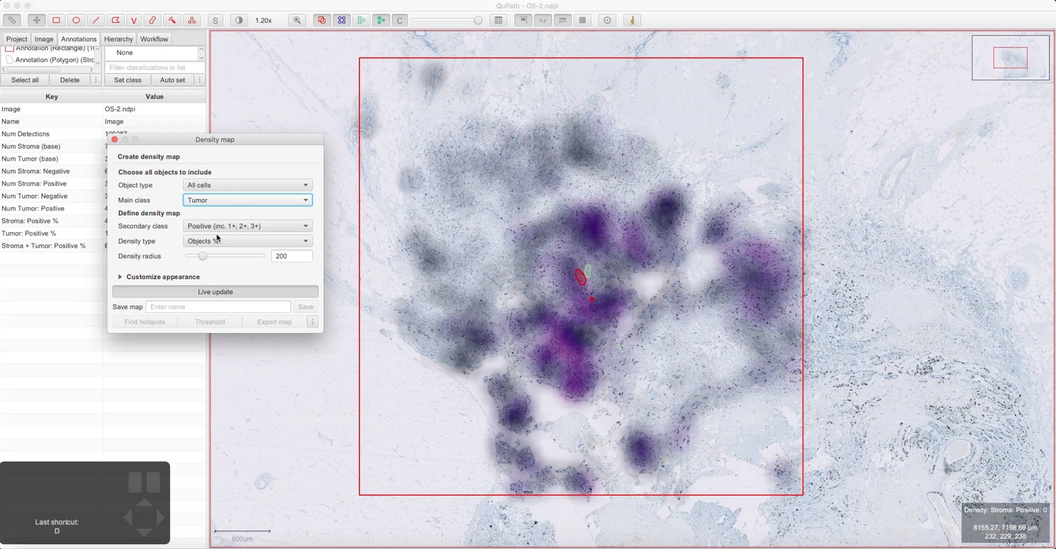
If I choose the Main class to be Tumor, then the density map will only include detections that are classified as Tumor.
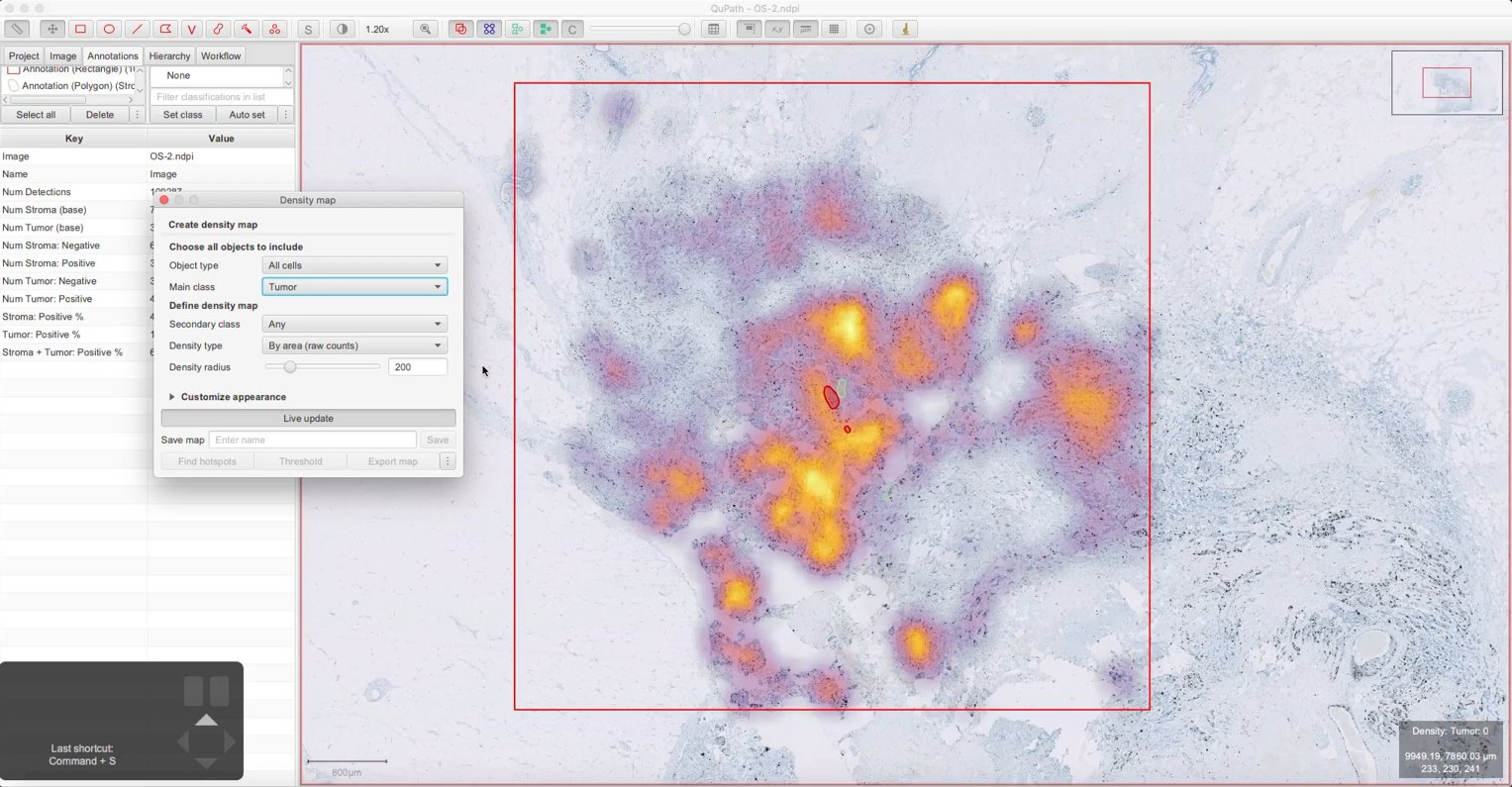
Density map showing tumor cells
Tip
Switching the Object type to All cells will make no difference here. This option exists for rare cases where you might have different kinds of detection object in the image (e.g. cells, and then subcellar structures within cells).
Tip
The location of a detection contributing to the density map is based on its ROI centroid. Density maps also support point annotations, in which case the individual points will be used.
Defining densities
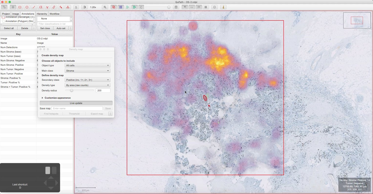
The Secondary class makes it possible to select a subset of objects that are of particular interest. This is optional – it can be left at Any if it isn’t needed.
A useful application of this here would be to look specifically at tumor cells classified as positive.
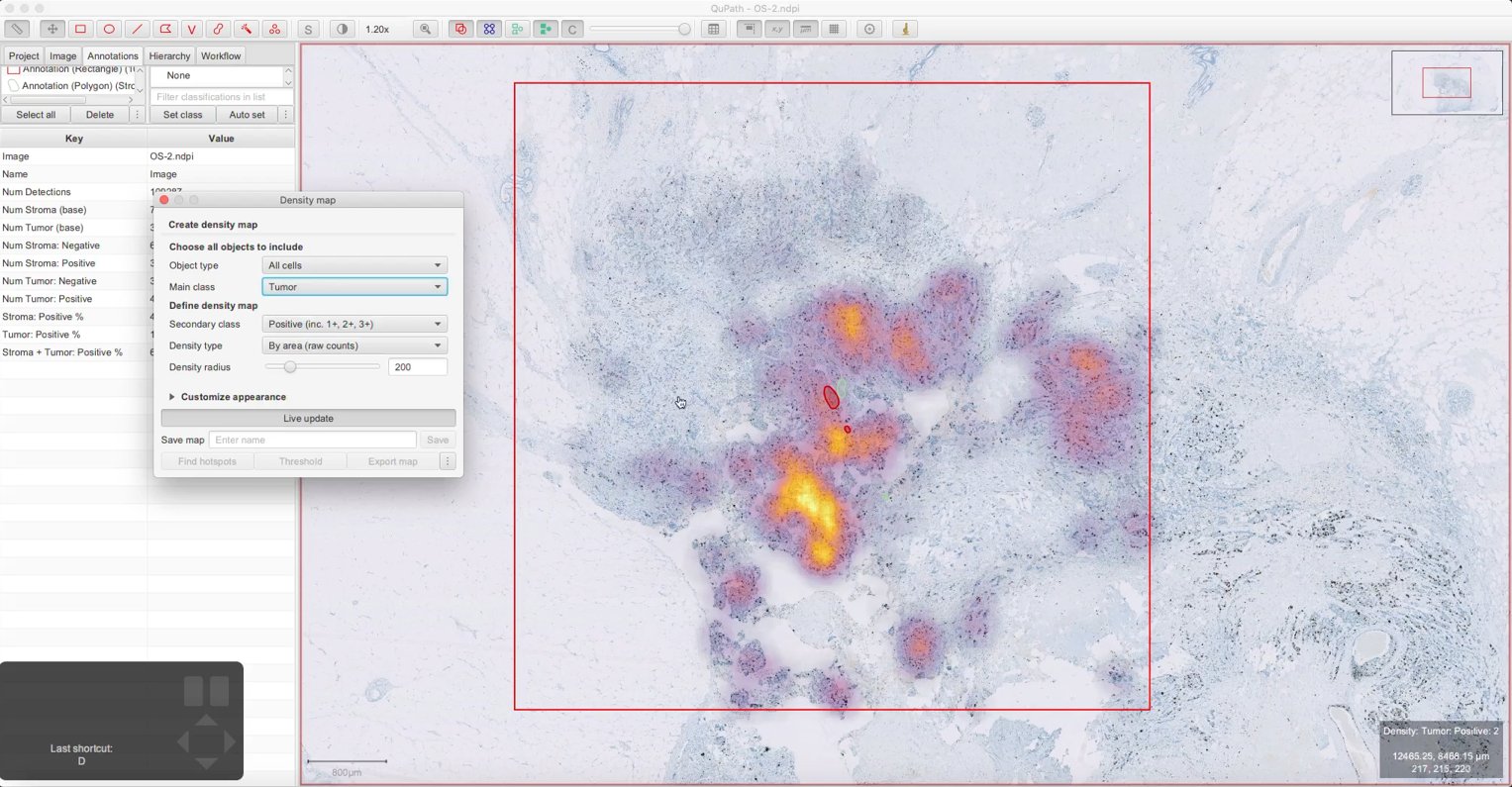
Density map showing positive tumor cells
This then works in combination with the Main class. If I switch that, I can look at the cells classified as both stromal and positive.
Density map showing positive non-tumor cells
I can also control how the densities are calculated using the Density type and Density radius.
By area (raw counts) – This means that each pixel in the density map represents the number of chosen objects within the defined radius. This is the default option.
Gaussian-weighted – Local densities are calculated using a weighted sum. This makes the exact values within the maps harder to interpret, but may be useful in some cases if the density map is used to generate other objects.
Objects % – Local densities are calculated by taking the number of objects within the radius that have both the Main class and the Secondary class, and dividing this by the number of objects with the Main class only.
In all cases, the radius is defined in calibrated units (i.e. µm, if available) and controls the resolution of the density map.
In the first two types, the densities are effectively normalized by area. In the last type, Objects %, the densities are normalized by objects.
We can use Objects % to calculate a local Ki67 labeling index: the percentage of tumor cells classified as positive.
Density map showing positive % tumor cells
Tip
You don’t have to use two classes. Often, the density of objects with a single classification is all you need.
In that case, it doesn’t really matter if you set that classification to be the Main class, Secondary class or both – QuPath will try to untangle them to create a suitable map.
Customizing the appearance
Expanding the Customize appearance panel provides various options to change the appearance of the density map, including the colormap. These are purely for visualization, and don’t influence the behavior of the map for thresholding or hotspot detection.
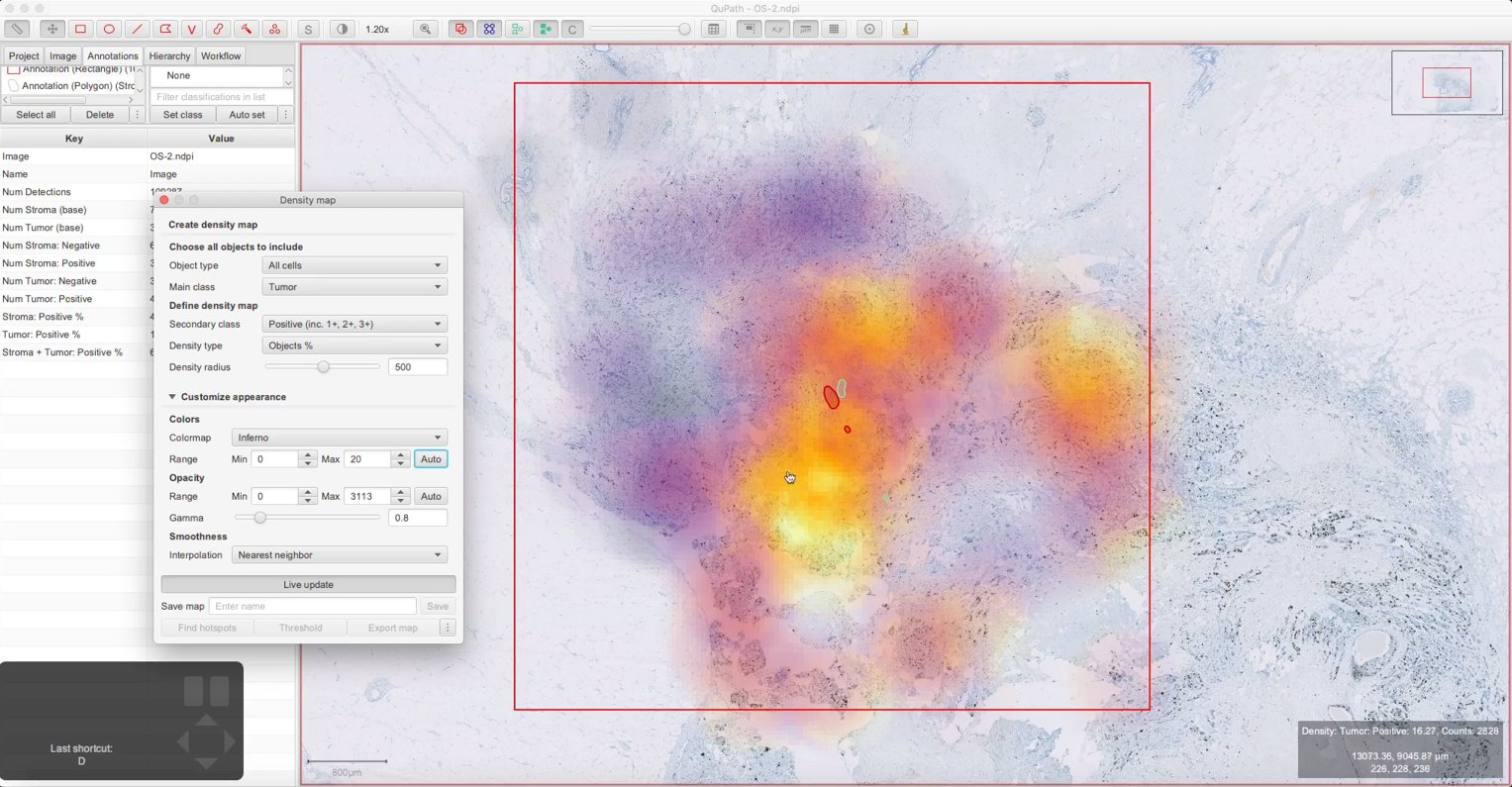
Density map showing positive % tumor cells with contrast adjusted
One thing to note is that the colors depend upon which objects meet both the Main class and Secondary class criteria.
The opacity does as well, except in the special case where using the Objects % option. This option can easily be influenced by outliers: in the Ki67 example, a single isolated positive tumor cell could give a density value of 100% (since there are no other objects nearby), but is probably a false positive and not be very meaningful. Usually, we want to consider only regions that have enough cells within them to be interesting. For that reason, the opacity in this case is based upon the Main class only, i.e. here it is the number of tumor cells.
This means that, by default, the density map for areas containing very few objects are usually almost transparent, and attention is drawn towards areas containing a lot of objects.
Tip
The Gamma slider makes it possible to adjust this opacity weighting. If you want to remove it altogether, set the gamma to 0.
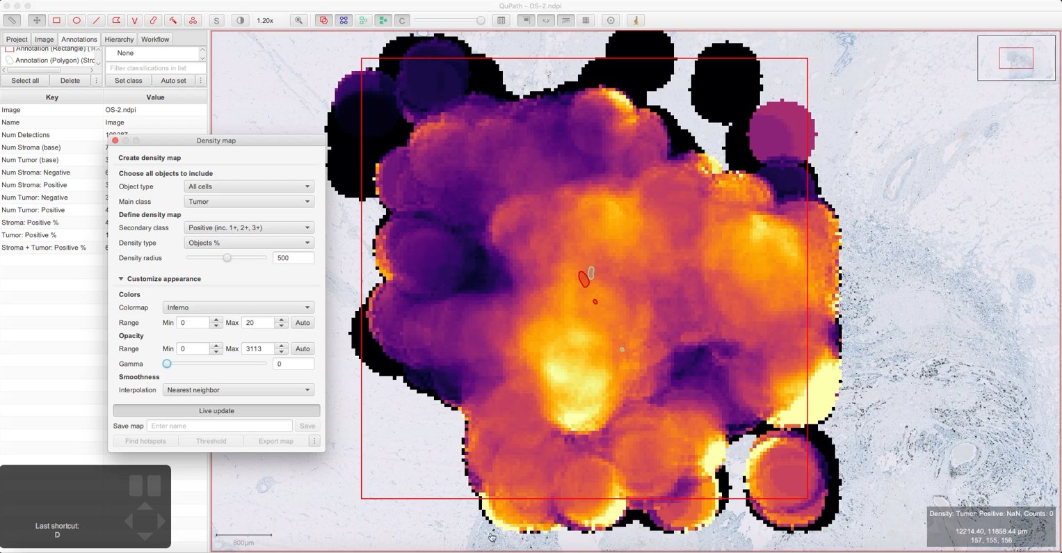
Density map showing positive % tumor cells with gamma = 0
Using density maps
The buttons at the bottom of the pane enable density maps to move beyond a visualization tool into becoming useful for analysis.
Save the density map
Before going further, you should really save your density map. This requires that you’re using a project (so there is a place to save the map).
This is essential if you want to use it within scripts later, and for that reason the subsequent buttons are disabled until after you’ve saved the map.
Tip
If you really want to override the need to save the map, and enable the buttons anyway, you can do this via the ⋮ button. However, you won’t be able to call the density map commands later in a script.
You can then use :Analyze –> Density maps –> Load density map to access the density map later and apply it to any image.
Find hotspots
A common use of density maps in pathology is to find ‘hotspots’: regions with a high density of something, however ‘density’ is defined.
Having customized your map using the options above, the Find hotspots button can be used to generate one or more non-overlapping hotspots based upon the highest values in the map. Each hotspot is a circular annotation with a radius that matches the radius option set when creating the map.
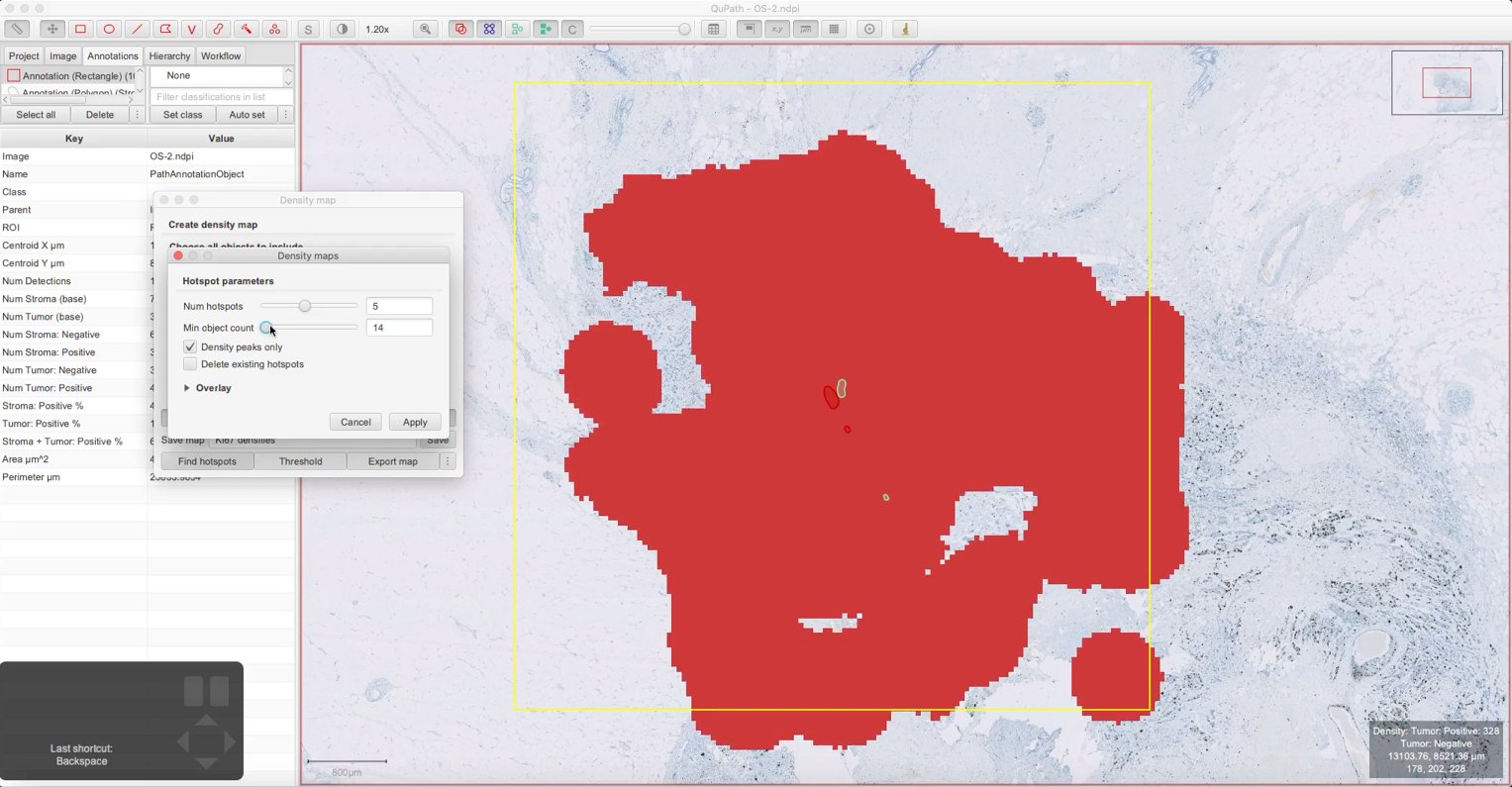
Density map hotspot thresholding
Hotspots can be generated within any annotations that are selected, or across the entire image if there is no selection. Some parameters are intuitive, but there are some important-but-not-obvious subtleties.
Num hotspots – This defines the maximum number of hotspots within the selected region (or full image). If the region is too small, a smaller number of hotspots may be returned.
Min object count – This can be used to exclude areas containing few objects from consideration, to avoid generating spurious hotspots that are really just due to outliers.
Density peaks only – In theory, one might expect a hotspot to be a ‘peak’ in the density map, where the density is higher than in surrounding pixels. In practice, the highest density within any region might not be a peak (because the peak is outside the region). On the other hand, removing the peak criterion could result in multiple hotspots being generated within a single large, high-density region. This option allows you to toggle whether a peak criterion is used or not.
Delete existing hotspots – This is handy when running the command multiple times, such as when tweaking parameters. It removes only hotspots with the same classification as the new hotspots being created.
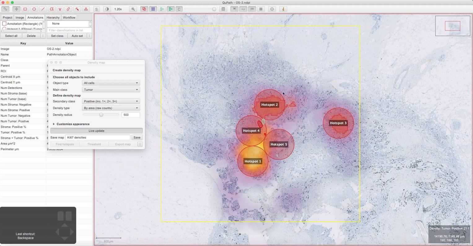
Density map hotspots
The name of the hotspot annotation reflects its ranking in descending order: if more than one hotspot is generated, the one name Hotspot 1 is the ‘hottest’ (i.e. corresponds to the highest density).
Tip
Because the dialog blocks the rest of QuPath, the Overlay pane makes it possible to adjust the overlay display – in case it wasn’t set nicely before pressing the Find hotspots button.
Density map resolution
Unless the image is very small, the density map is calculated at a lower resolution than the full image. The hotspot calculations are ‘rasterized’, meaning they work on pixels in the lower resolution density map. This imposes a limit on the accuracy.
Once the hotspot is created, the object counts QuPath makes inside the annotation are no longer limited by the density map resolution. This means that the number of objects counted in the hotspot may not be identical to the value in the density map.
It also means that slightly shifting the hotspot (by a distance lower than the density map resolution) can sometimes give a slightly higher value. In this way, the command really provides an efficient estimate of hotspots, rather than precise locations from an exhaustive search – but any differences can be expected to be small.
Threshold
Another use of a density map is to convert detections to annotations.
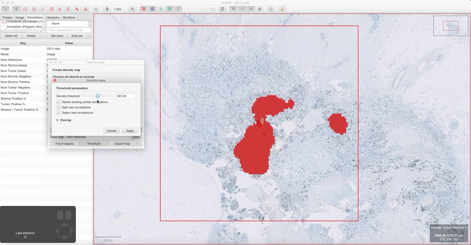
Density map thresholding
For example, this can be used to generate an annotation surrounding an area containing mostly tumor cells, along with other cell types. I imagine this could be worthwhile in assessing tumor infiltrating lymphcytes, avoiding the need for extensive manual annotation or pixel classification.
Density threshold – Minimum density
Min object count – Only available when using Objects %; this can be used to exclude areas containing few objects from consideration, to avoid generating spurious hotspots that are really just due to outliers.
Delete existing similar annotations – Useful when running the command multiple times to refine parameters.
Select new annotations – Useful when you want to do something immediately with the annotations that were created. This is most helpful within scripts.
Export map
Finally, density maps can be export for use elsewhere – or sent to ImageJ for further processing.
Note that the Color overlay option includes only the density map, and not the underlying image pixels. This is useful if you want a translucent PNG for superimposing elsewhere.
If you want to export the image as it appears in the viewer, use instead .